6 The End-to-end Workflow: A recap

In this chapter:

We will do a recap of everything we have learned until now.

I. Environment Setup

Step 1: Open the Project folder in VS Code

Go to File –> Open Folder.

Step 2: Start Julia REPL

Press Cmd + Shift + P (Mac) / Ctrl + Shift + P (Windows), and then search for Julia: Start REPL. Hit enter to choose the option from the dropdown menu

Step 3: Activate Project Environment

Go to package manager mode. (Press ] while in Julia REPL to go to Package Manager mode). Then type activate . and hit enter. Now you should see your project folder name instead of (@v1.7) pkg>.
Return to Julia REPL mode by hitting backspace

Step 4: Create new Julia file for your project

Go to File –> New File
Save the file with a name you like. To save the file you can do Cmd + S / Ctrl + S.

Step 5: Make sure you have the required packages

using Pkg
Pkg.status()

CSV
DataFrames
PyPlot
ScikitLearn

If some packages are missing, you’ll get an error in the next step.

Step 6: Load the packages

using DataFrames
using CSV
using ScikitLearn
using PyPlot

II. Data

Step 7: Load the Data

pathtodata = joinpath(pwd(), "diabetes.csv")
data = CSV.read(pathtodata, DataFrame);

Instead of diabetes.csv, pass your dataset name.

Step 8: Inspect the data columns

first(data,5)

5 rows × 8 columns

	npreg	glu	bp	skin	bmi	ped	age	type
	Int64	Int64	Int64	Int64	Float64	Float64	Int64	String3
1	6	148	72	35	33.6	0.627	50	Yes
2	1	85	66	29	26.6	0.351	31	No
3	1	89	66	23	28.1	0.167	21	No
4	3	78	50	32	31.0	0.248	26	Yes
5	2	197	70	45	30.5	0.158	53	Yes

If you find columns that are redundant or meaningless, delete those columns. For example, suppose we had a meaningless column called RowNo. To delete the column you can use the command data = select(data,Not(:RowNo)). Make sure you only run the delete command once per column. Trying to run it multiple times will give you an error.

Step 9: Extract the features and target

X = Array(data[!,Not(:type)]);
y = Array(data[!, :type]);

Instead of :type in the above code, you should use the column name you have for your target.

III. Model Training

Step 10: Split the data into training set and test set.

@sk_import model_selection: train_test_split;
X_train, X_test, Y_train, Y_test = 
    train_test_split(X, y, test_size=0.2, 
        random_state=42);

Here I chose 20% for test set (so 80% of the actual data will be used for training).

Step 11: Build a baseline model

Before going into complicated models, it’s recommended that you try a simple model first. You’ll call this your baseline model. In our case, we’ll have a simple logistic regression model our baseline.

@sk_import linear_model: LogisticRegression;
simplelogistic =LogisticRegression();

fit!(simplelogistic, X_train, Y_train);

Step 12: Check the accuracy of your baseline model

@sk_import metrics: accuracy_score

Y_pred_train = predict(simplelogistic,X_train);
print(accuracy_score(Y_train,Y_pred_train))

0.7886792452830189

Step 13: Create a slightly complicated model and check its accuracy

We’ll have a shallow neural network with one hidden layer and 5 nodes as our slightly complicated model.

@sk_import neural_network: MLPClassifier;
simpleneuralnetwork = MLPClassifier(hidden_layer_sizes=(5));

fit!(simpleneuralnetwork, X_train, Y_train);

Y_pred_train = predict(simpleneuralnetwork,X_train);
print(accuracy_score(Y_train,Y_pred_train))

0.30943396226415093

Step 14: Search the model space for better hyperparameters with 3-Fold cross validated training

using ScikitLearn.GridSearch: GridSearchCV
gridsearch_logistic = GridSearchCV(LogisticRegression(),
            Dict(:solver => ["newton-cg", "lbfgs", "liblinear"], 
            :C => [0.01, 0.1, 0.5, 0.9]))

fit!(gridsearch_logistic, X_train, Y_train);

:C is a regularization parameter.
For more hyperparameters that are tweakable, please refer to LogisticRegression’s ScikitLearn documentation page.

Print the results of hyperparameter search

gridsearch_logistic_results = DataFrame(gridsearch_logistic.grid_scores_);
hcat(DataFrame(gridsearch_logistic_results.parameters), 
    gridsearch_logistic_results)[!,Not(:parameters)]

12 rows × 4 columns

	solver	C	mean_validation_score	cv_validation_scores
	String	Float64	Float64	Array…
1	newton-cg	0.01	0.8	[0.764045, 0.829545, 0.806818]
2	lbfgs	0.01	0.8	[0.764045, 0.829545, 0.806818]
3	liblinear	0.01	0.720755	[0.696629, 0.715909, 0.75]
4	newton-cg	0.1	0.796226	[0.775281, 0.806818, 0.806818]
5	lbfgs	0.1	0.796226	[0.775281, 0.806818, 0.806818]
6	liblinear	0.1	0.735849	[0.719101, 0.704545, 0.784091]
7	newton-cg	0.5	0.784906	[0.775281, 0.772727, 0.806818]
8	lbfgs	0.5	0.784906	[0.775281, 0.772727, 0.806818]
9	liblinear	0.5	0.739623	[0.707865, 0.727273, 0.784091]
10	newton-cg	0.9	0.792453	[0.775281, 0.772727, 0.829545]
11	lbfgs	0.9	0.792453	[0.775281, 0.772727, 0.829545]
12	liblinear	0.9	0.754717	[0.730337, 0.738636, 0.795455]

The best model from the grid search will be saved in best_estimator_ field of your grid search training results.

best_logistic_model = gridsearch_logistic.best_estimator_

PyObject LogisticRegression(C=0.01, solver='newton-cg')

Step 15: Repeat GridSearchCV for other models you have

Just don’t simply use the list of numbers I have used for the hidden_layer_sizes. It might make sense to have 1000s of nodes and many hidden layers if you are doing image processing.

Sometimes, you might have to do multiple grid search rounds with different hyperparameter settings to find the most optimal values.

gridsearch_neuralnet = GridSearchCV(MLPClassifier(),
            Dict(:solver => ["sgd", "lbfgs", "adam"], 
            :hidden_layer_sizes => [(2), (20), (1,5,10), (10,10), (10,20,10)]))
fit!(gridsearch_neuralnet, X_train, Y_train);


gridsearch_neuralnet_results = DataFrame(gridsearch_neuralnet.grid_scores_);
hcat(DataFrame(gridsearch_neuralnet_results.parameters),
    gridsearch_neuralnet_results)[!,Not(:parameters)]

15 rows × 4 columns

	solver	hidden_layer_sizes	mean_validation_score	cv_validation_scores
	String	Any	Float64	Array…
1	sgd	2	0.562264	[0.685393, 0.306818, 0.693182]
2	lbfgs	2	0.690566	[0.685393, 0.693182, 0.693182]
3	adam	2	0.596226	[0.685393, 0.784091, 0.318182]
4	sgd	20	0.686792	[0.662921, 0.693182, 0.704545]
5	lbfgs	20	0.709434	[0.730337, 0.681818, 0.715909]
6	adam	20	0.683019	[0.707865, 0.704545, 0.636364]
7	sgd	(1, 5, 10)	0.543396	[0.674157, 0.647727, 0.306818]
8	lbfgs	(1, 5, 10)	0.690566	[0.685393, 0.693182, 0.693182]
9	adam	(1, 5, 10)	0.686792	[0.685393, 0.681818, 0.693182]
10	sgd	(10, 10)	0.660377	[0.662921, 0.693182, 0.625]
11	lbfgs	(10, 10)	0.716981	[0.707865, 0.693182, 0.75]
12	adam	(10, 10)	0.630189	[0.629213, 0.693182, 0.568182]
13	sgd	(10, 20, 10)	0.683019	[0.58427, 0.715909, 0.75]
14	lbfgs	(10, 20, 10)	0.750943	[0.707865, 0.772727, 0.772727]
15	adam	(10, 20, 10)	0.690566	[0.662921, 0.670455, 0.738636]

best_neuralnetwork_model = gridsearch_neuralnet.best_estimator_

PyObject MLPClassifier(hidden_layer_sizes=(10, 20, 10), solver='lbfgs')

Step 16: Compare the results of competing models on test set

@sk_import metrics: accuracy_score
Y_pred_test_logistic = predict(best_logistic_model, X_test)
logistic_accuracy = accuracy_score(Y_test,Y_pred_test_logistic)

Y_pred_test_neural = predict(best_neuralnetwork_model, X_test)
neural_accuracy = accuracy_score(Y_test,Y_pred_test_neural)

models = ["logistic","neural"]
scores = [logistic_accuracy, neural_accuracy]
# Plotting the results 

using PyPlot  
figure()
b = PyPlot.bar(x = models, height = scores*100);
xlabel("Models"); 
ylabel("Accuracy Score");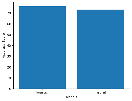

Here we have used accuracy for comparison. You can also use precision, recall, or f1 score in a similar fashion for comparing models, depending on the domain of prediction.

Step 17: Save your best model for production

The model you found to be the best performing one can be saved to the disk so that you don’t have to train your models every time you restart Julia or you want to make predictions. We’ll need three packages to save a scikit-learn model: PyCall, PyCallJLD, and JLD

using PyCall, JLD, PyCallJLD
save("saved_file.jld", "diabetic_prediction", best_logistic_model)

The save function takes three arguments: the name of the file, the name you want to give to the model, the trained model.

To load a saved scikit-learn model, you can use the load function:

logistic_model = load("saved_file.jld", "diabetic_prediction")

PyObject LogisticRegression(C=0.01, solver='newton-cg')

Now let’s check if our loaded model is working.

predict(logistic_model, X_test)[1:4]

4-element Vector{Any}:
 "No"
 "No"
 "No"
 "No"